DRAFT: Generating random unit vectors
Generation of a random unit vectors in \(D\) dimensions is a common requirement. Perhaps you want to simulate some kind of random walk through space. How can we generate vectors such that their direction is uniformly distributed?
Let’s store the components in a \(D\) dimensional array, in C we could do something like
double vec[D];
for (int i = 0; i < D; i++)
    vec[i] = rand();
where rand is some function that generates a double in the range \([-1,1]\).
Easy, problem solved. Well, almost. We said that we wanted a unit vector, so we should normalize the vector, then we’re done.
double length = 0;
for (int i = 0; i < D; i++)
    length += vec[i] * vec[i];

length = sqrt(length);

for (int i = 0; i < D; i++)
    vec[i] /= length;
Ok, so even with normalisation that was pretty easy. But are the results actually any good? Let’s take a closer look at the distribution of the values, we’ll do this by looping the above code 2,000,000 times with \(D=3\) and plotting the resultant points in Python. The results are visible in figures 1 and 2.
Figure 1 shows the distribution over the sphere when viewed front on, figure 2 shows the same but with the sphere unwrapped using a Lambert azimuthal equal-area projection, which I have covered in another post. To make a long story short, this projection allows us to see the entire surface of the sphere without ruining our view of the density of points. From now on I will stick to showing just the Lambert projections.
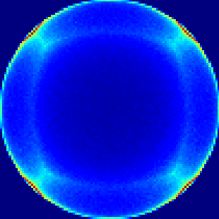
front view
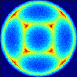
Lambert projection
We can see clearly in figure 2 that we have a very non-uniform distribution. To understand why lets take a step back to \(D=2\). The problem arises because we generate our coordinates in a square and then normalise them onto a circle. For the vectors that naturally lie inside the circle this is not a problem, they are just stretched a bit during normalisation until they lie on the edge of the circle. But what about vectors that naturally lie outside the circle? Here is an example set of points

Clearly this is not rotationally symmetric, we have all of these extra points in the corners which aren’t there at the sides. After normalising we will end up with points bunching up in the corner regions as all of these extra points are squeezed down onto the circle - not uniformly distributed at all!
Ok, so what can we do about it? Still in \(D=2\), lets try polar coordinates. We generate an angle \(\theta\), then the corresponding point on the circle is \((\cos\theta,\sin\theta)\).
Its difficult to visualise this but we know it works because a differential element around the circumference of the circle is \(dC=r d\theta\). Clearly if we can generate \(\theta\) uniformly we will get a uniform distribution around the circumference as a result.
Ok, so lets take the same idea and apply it for \(D=3\). In this case, we now generate two angles, \(\theta\) and \(\phi\), and the corresponding point on the surface of the sphere is given by \((\sin\theta\cos\phi, \sin\theta\sin\phi,\cos\theta)\) where we adopt the convention that \(\phi\) is the polar angle and \(\theta\) is the azimuthal angle. Let’s generate points again and see what we get.
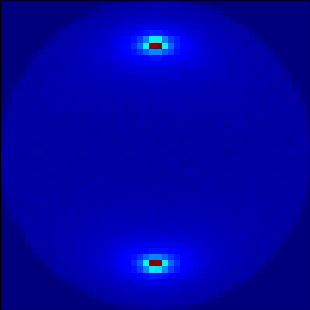
spherical polar coordinates
It certainly looks a lot nicer, but we get some very hot spots at the poles. Let’s examine the differential again, this time a surface area differential element is given by
\[\begin{equation} dA = r \sin\phi\; d\phi\; d\theta \end{equation}\]The feature to notice is that \(dA \propto sin\phi\). This means that if we take a particular \(d\theta\) and \(d\phi\) the area to which they correspond will be smaller for values of \(\phi\) near \(0\) and \(\pi\) (i.e. where \(\sin\phi\) is smallest). As \(\phi\) is the polar angle the result is a large bunching of points near the poles of the sphere. The point illustrated here is that just because something works nicely in a particular dimension (in this case \(D=2\)), doesn’t mean that it can be easily generalised to other dimensions.
A simple general solution
Ok so now we know the problem, but what can we do about it? Maybe the simplest solution might be the best. Refer back to figure 3, where we could see the problem of having extra points in the corners of the box in which we generate our points. All we really need to do is ignore these points, we can do this by simply drawing again if the vector we get is outside the sphere.
double vec[D];
double length = 0;

do
{
    for (int i = 0; i < D; i++)
        vec[i] = rand();

    for (int i = 0; i < D; i++)
        length += vec[i] * vec[i];

} while (length > 1);

length = sqrt(length);
for (int i = 0; i < D; i++)
    vec[i] /= length;
There is the obvious disadvantage that we are wasting time generating points that we don’t actually need. In two dimensions about 21.5% of points that we generate are outside the circle, in three dimensions this increases to about 47.6%.
Without going into detail, the volume on a unit \(n\)-ball for arbitrary \(n\) is given by
\[\begin{equation}\label{volume-n-ball} V_n=\frac{\pi^\frac{n}{2}}{\Gamma(\frac{n}{2}+1)} \end{equation}\]and the volume of a box containing it is simply
\[\begin{equation}\label{volume-n-box} V_n=2^n \end{equation}\]We can plot these and see that while (quite counter intuitively) the volume of the sphere never gets particularly large with dimension, the volume of the box containing it is highly divergent.

n (bottom line) and the volume of a box containing it (top line)
It’s worth noting that comparison of “volume” between dimensions doesn’t make a whole lot of sense, we really can only compare the values of the two lines at any given point. We can do that clearly by considering the ratio between the two volumes. The percentage of points that we keep is vanishingly small for large dimension.

volume of a box containing it with respect to n
So lets take a look at the run time, by comparing the time taken to draw from the whole cube (which we know is not correct), compared to using this method of discarding corner points.
I wanted to plot this over the same ranges as figures 5 and 6 but the time taken as we get to higher \(D\) is so astronomical that there’s not really any point. Instead I will just plot up to \(D=6\).

using box draw (bottom line) and discard corners (top line)
From equations \(\eqref{volume-n-ball}\) and \(\eqref{volume-n-box}\) we can quickly see that the by just \(D=115\) the chance of successfully drawing a point inside the sphere is equivalent to picking one atom out of all atoms in the observable universe (\(\approx 10^{82}\)).
If you only need less that 6 or so dimensions then discarding the corners is probably going to be ok, after all <15 seconds for 10 million vectors isn’t that bad, right?
Lambert
Yeah, ok, but what if I do need 115 dimensions? I honestly don’t know any specific case where you would but for sure its very common for physical problems to have high dimensional parameter spaces (not usually spatial dimensions but lets investigate anyway).
We spoke earlier about the Lambert azimuthal equal-area projection. We can actually use this in reverse to generate our points. Effectively (in \(D=3\)) we generate points on a disc and map them back to the sphere.
The mapping (again, see my last post, which includes demonstration of the equal area property) is given as follows
\[\begin{equation}\label{lambert-cartesian} (X,Y)=\left( \sqrt{\frac{2}{1-z}}x, \sqrt{\frac{2}{1-z}}y \right) \end{equation}\]Which we can easily invert
\[\begin{equation}\label{inverse-lambert-cartesian} (x,y,z)=\left( \sqrt{\frac{1-z}{2}}X, \sqrt{\frac{1-z}{2}}Y, z \right) \end{equation}\] \[\begin{equation}\label{inverse-lambert-2d} (x,z)=\left( \sqrt{\frac{1-z}{2}}X, z \right) \end{equation}\] \[\begin{equation}\label{inverse-lambert-super} (x,y,z)=\left( \sqrt{\frac{1-z}{2}}\sqrt{\frac{1-z}{2}}z, \sqrt{\frac{1-z}{2}}z, z \right) \end{equation}\]And we may take polar coordinates
\[\begin{equation}\label{inverse-lambert-polar} (x,y,z)=\left( \sqrt{\frac{1-z}{2}}\cos\theta, \sqrt{\frac{1-z}{2}}\sin\theta, z \right) \end{equation}\]where \(\Theta=\theta\) and \(R=\sqrt{\frac{1-z}{2}}\) (capital coordinates on the disc and lower case on the sphere). We simply generate \(\theta\) and \(z\) and get coordinates on the sphere through the above expression.
At the moment this only works in \(D=3\), so lets examine the run time here.

using inverse Lambert (bottom line) and discard corners (top line)
This is good, the inverse Lambert method is significantly faster in \(D=3\) than the discard corners method. Unfortunately at the moment this is the only dimension it works in. We’re going to need to think a bit more about how to generalise it.
Look back at equation \(\eqref{inverse-lambert-cartesian}\), can we make a guess as to what a higher dimensional form might look like? It’s not that much of a stretch to imagine it might look like
\[\begin{equation}\label{inverse-lambert-cartesian-general} (x_1,x_2,\cdots,x_{n-1},z)=\left( \sqrt{\frac{1-z}{2}}X_1, \sqrt{\frac{1-z}{2}}X_2, \cdots, \sqrt{\frac{1-z}{2}}X_{n-1},z \right) \end{equation}\]To keep things a little simpler, lets consider just \(D=4\) for a bit,
\[\begin{equation}\label{inverse-lambert-cartesian-4} (x_1,x_2,x_3,z)=\left( \sqrt{\frac{1-z}{2}}X_1, \sqrt{\frac{1-z}{2}}X_2, \sqrt{\frac{1-z}{2}}X_3,z \right) \end{equation}\]We’re left with the problem of generating \(X_1\), \(X_2\) and \(X_3\).